Predicting Myers-Briggs Type Indicator Test (MBIT) personality type

16 MBIT personality types

What is MBIT?

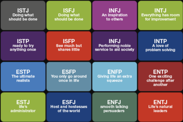
MBIT is a questionnaire system, created in 1944,The test is used to predict the personality of person which is defined by 8 individual type of personalities which are:

E=Extrovert,I=Introvert,S=senstive ,N=Intuitive, T=Thinking,F=feeling ,J=juding ,P=percieving.These 8 types can be grouped into 4 major class of personalities where classes can be whether a person is:

• Extrovert or Introvert(E or I)
• Sensitive or Intuitive(S or N)
• Thinking or Feeling(T or F)
• Judging or Perceiving(J or P)

but not both .In this way a person has one of the personality from each 4 classes there by making 16 possible combination of 4 personalities like ESTJ which means the person has extrovert, Sensitive, Thinking and Judging type of personality .The test is quite popular and is widely used in different areas like classrooms, job hiring , psychological analysis.

4 major MBIT personality type

This blog will explain how can we predict these 16 MBIT personalities using machine learning and deep learning models.

Data

The (MBTI) Myers-Briggs Personality Type Dataset is taken from the kaggle. The dataset has content written by different people on the web. Our dataset has 8600 rows i.e. the content written by 8600 people is recorded . With each row there are 50 things , they have either posted or content viewed like webpages , Youtube pages all seperated by ’ — — — ’ . Along with the content section , there is MBTI code/ type i.e. the predictor of the dataset, which indicates that this person has 4 personality type.

Class Distribution

Pre Processing

• Cleaning URL : For cleaning URL present in the samples , we have used regular expression . In this phase , we removed URL by none.
• Cleaning punctuations : To remove the punctuations from the data, we have used regular expression.
• Tokenization : The content of each person is converted into bag of tokens.
• Stop word Removal : From the token of words , the stop words are removed. Stop words are the most common word in the text which is needed to be removed to get the important word will get the focus.
• Stemming : The token word is needed to be stemmed, to get the base word . Stemming is mainly done to create index of words.

Feature Extraction

• PCA (principle component analysis) 1000 features were extracted from 77000 features(terms) in tfidf matrix using decomposition.pca sklearn library.
• N-Gram the features are created with bi-gram . From the corpus of training data , the two adjacent were taken .The bi-gram features makes the data more interesting . The more detailed version with implementation is explained in the Language model subsection.
• LSA (Latent Semantic Analysis) extracted similarity values of each person with all 8 classes E,I,S,N,T,F,J,P. hence using these 8 features one class from E,I ,one class from S,N ,one class from T,F and 1 class from J,P is predicted. this is thoroughly explained in language section model.

Models Applied for Prediction

Machine Learning Models

• TFIDF Based Prediction: tf-idf stands for Term frequency-inverse document frequency. Its is a weighting scheme that assigns each term in a document a weight based on its term frequency (tf) and inverse document frequency (idf). The terms with higher weight scores are considered to be more important and will try to classify according to them. Normalized Term Frequency (tf) defines number of times the term t appear in each document d , here d is considered to a person 50 posts.

Normalised term frequency (tf) = tf(t,d) / length(d). 
Inverse Document Frequency (idf) : N/N(t) 
where, 
N =Total number of post 
N[t] =Number of post containing term t.

• SGDclassifier : Stochastic Gradient Descent(SGD) is an optimization algorithm used to find optimal values of parameters by using gradient(slope).The Sgdclassifier learns linear classification using loss functions like SVM, Logistic Regression and updates parameter using SGD which used only some random samples instead of whole dataset to update parameters. Here we have used SGD with logistic regression by specifying ”log” in loss parameter of the classifier. loss function used=logistic regression :

h(Q)   = 1/(1 + e -QTx ) (1)

• Gaussian Naive Bayes model is trained on 70% train data and tested on 30% data. the model is applied on whole tfidf matrix and after extracting pca features. on whole tfidf model model accuracy was 12% and on pca accuracy decreased to 6%.
• K Nearest Neighbor 7 neighbors were used to find the neighbors and taking majority vote. on whole tfidf model model accuracy was 15.01% and on pca accuracy increased to 15.05%.

Ensemble Models

Ensemble models are models that uses many classifiers to get the predictions .they are more accurate than normal ml models as thy take into account different classifiers.They also remove biasness and variance. here we have used one bagging and one boosting models described as below.

• Boosting Boosting is an ensemble modeling technique which attempts to build a strong classifier from the number of weak classifiers. For our dataset we made use of Adaboost algorithm.
• Bagging Bagging is an ensemble meta-estimator that makes estimation multiple times on the random subset of the original data and then aggregate individual prediction by voting or averaging to find the final decision. The bagging method is applied on the extracted by LSA and estimator are set to 10. To make use of bagging we made use of sklearn ensemble class and imported the bagging classifier.

Lexical and Semantic Analysis

For analysing lexical and semantic of data we applied NLP models like a lexical model N gram that analysed the syntactic part of the data that is it tried predicted words based on syntax like words behind it and to analyse semantics of the data we applied LSA which deals with meaning/concept of the data.

• N-Gram To implement Bi-gram model we find created the bi-gram features of both training and testing dataset. below features are extracted from the training dataset: 1. Bi-grams of the class 2. Unique words in the class To find the probability of a word and a bi-gram in Extroversion-Introversion is calculated as:

1. if bigram is in the class as well as word in the unique word of class then p(wi,wi-1) = C(wi,wi-1)/(C(wi)+len(vocab)) 
2. if bigram is not in the class as well as word in the unique word of class then p(wi,wi-1) = 1/(C(wi)+len(vocab)) 
3. p(wi,wi-1) = 1/len(vocab)

LSA Latent Semantic Analysis(LSA) is a Topic Modelling Technique used to find topics in a collection of documents by grouping semantically similar words in a topic .Words that are similar in context of their meaning is assigned similarity score of 1 and similarity measure varies from 0–1. we implemented LSA here by creating 8 tfidf matrices by extracting person with each class (E,I,S,N,T,F,J,P) to have sematically similar words in each topic.Then we used a library function TrucatedSVD(singular vector division) to decompose above each matrix into 3 matrices ( 1:documenttopic,2:topic-topic ,3:topic-term their multiplication gives the semantic score). Thus with input as first matrix,5000 word,2 topics we got 2 topics of semantically similar words then by manual identification we selected 1 topic with more number of words similar to that class given one class from each E/I,S/N,T/F,J/p based on highest similarity score.

score=E(similarity score of words matched in a topics)

Results

Accuracy of each model

Conclusion

Features are extracted by PCA, LSA and N-gram. Among Multinomial model Naive Bayes and KNN , KNN gave better results as compared to Naive Bayes. Among different Ensemble methods (Bagging and Boosting ) , Bagging gave better results than Boosting. To analyse the semantic and analysis of the data, N-gram and Lsa language models are used, out of which LSA out performed. Hence we induced that features created from tfidf , features extracted by LSA along with Bagging gave the best results.

Acknowledgment

We would like to acknowledge the guidance and support of our mentor Dr. Tanmoy Chakraborty and TA’s ( Shiv Kumar Gehlot, Chhavi Jain ,Shikha Singh,Pragya Srivastava,Vivek Reddy,Nirav Diwan,Aanchal Mongia,Ishita Bajaj) for the successful completion of our project under the subject Machine Learning in our college IIIT Delhi.#MachineLearning2020

Reference

• Golbeck, J.; Robles, C.; Edmondson, M.; Turner, K. Predicting personality from Twitter. In Proceedings of the IEEE Third International Conference on Privacy, Security, Risk and Trust and IEEE Third International Conference on Social Computing, Boston, MA, USA, 9–11 October 2011. Available online: https://ieeexplore. ieee.org/document/6113107/ (accessed on 25 August 2018)
• Machine Learning Approach to Personality Type Prediction Based on the Myers–Briggs Type Indicator,School of Computing and Digital Media, London Metropolitan University, London N7 8DB, UK;h.kazemian@londonmet.ac.uk,2020
• Assessment of Latent Semantic Analysis (LSA) text mining algorithms for large scale mapping of patent and scientific publication documents.Tom Magerman, Bart, Van Looy , Bart Baesens,Koenraad Debackere,October 2011.
• Predicting Sentences using N-Gram Language Models.January 2005,Conference: HLT/EMNLP 2005, Human Language Technology Conference and Conference on Empirical Methods in Natural Language Processing, Proceedings of the Conference, 6–8 October 2005, Vancouver, British Columbia, Canada

Individual Contributions

1. Era Sharma- MT19121 :- Pre processing, Literature survey , TFIDF ,SGD classifier , Feature Extraction using LSA, Multinomial KNN, Latent Semantic Analysis(LSA) model
2. Mansi Sharma-Mt19092:- Pre Processing, Literature survey, TFIDF , Feature Extraction using N-gram, N-Gram Model , bagging and boosting
3. Deepak Thakur-2017337 :- Decision tree, Feature Extraction using PCA, Multinomial Naive Bayes.